A swaption is an option that gives the possibility to its owner to enter in a swap at a predetermined fixed rate K.
We note B(t, T) the discounting curve. We consider a swap with a maturity 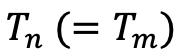 .
.
We have :
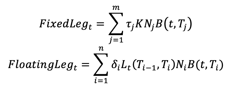
The swap rate is the rate that makes the two legs of the swap equal:
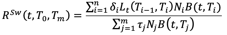
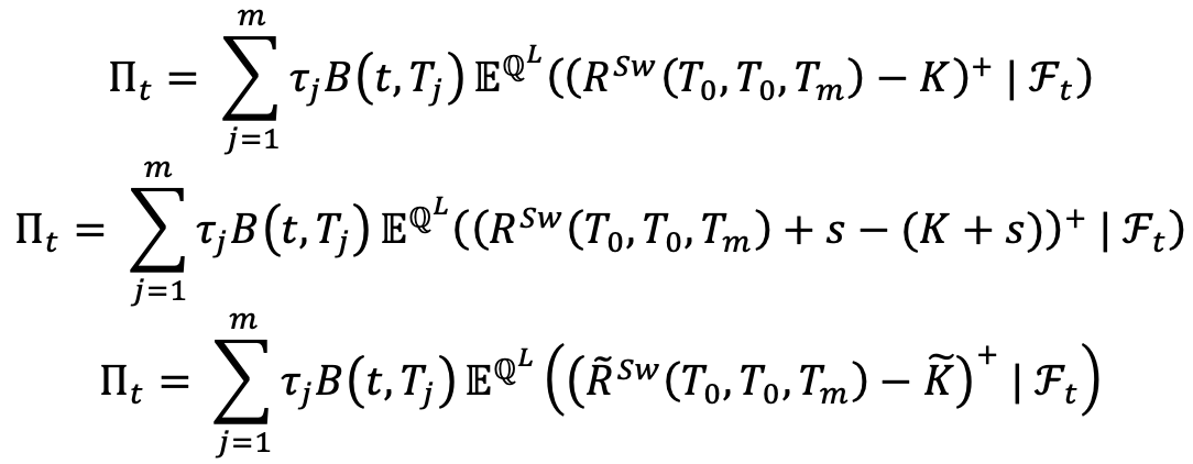
The payoff of the paying swaption is:
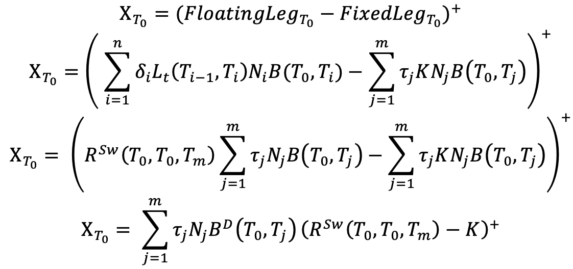
Where:  .
.
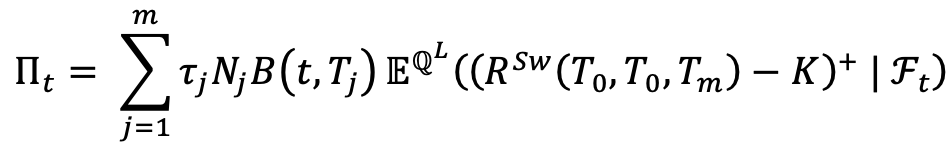
Thanks to the fundamental formula of pricing we have that the price of the swaption, that can be exercised in  , at the instant
  is:
is:
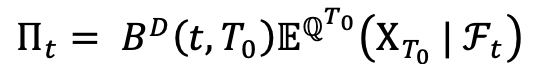
Where  is the probability associated with the numeraire
  .
.
We now write the price of the swaption under the numeraire 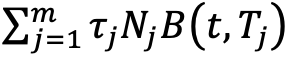 (which is often called Level). With the classic change of numeraire formula, we have:
The swaption can be seen as a Call on the swap rate with a strike K.
For the currencies with non-negative swap rates, e.g. USD and GBP, the market practice is to consider that the forward swap rate follows a Black log-normal diffusion under the probability Level  :
:
![]()
With: 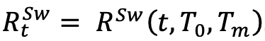
With this model, it is easy to price a swaption with the well known Black formula:
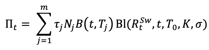
With:
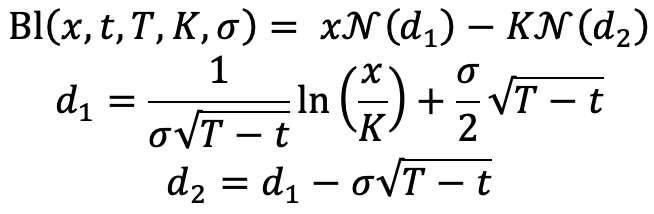
where  is the cumulative normal distribution function.
The only unknown is the volatility  . The market provides volatilities for swaptions with different durations for the underlying swaps (1Y, 2Y, 5Y, 10Y, 20Y, etc.) and with different exercise times (1M, 3M, 6M, 1Y, 2Y, 5Y, 15Y, etc.).
For each duration and each exercise time, we have volatilities for different strikes. We want a complete volatility smile to have a volatility for any strike. To do this, we suppose that the forward swap rate follows a SABR diffusion:
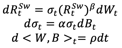
The reason why we use the SABR model, and why it is world-famous, is that it gives a (nearly) close formula for the implied volatility. Let’s note 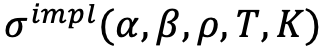 the SABR-implied volatility. The idea is then to calibrate the parameters of our model
 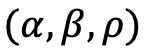 on the market volatilities. We do this for each exercise time and for each duration. A classic way to do this calibration is to minimize the following function:
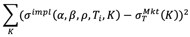
for each T = 1M, 3M, 6M, 1Y, ..., 15Y, ...
After this calibration, we have a smooth volatility curve, the function of the strike, for each exercise time and each underlying swap’s duration. To finish, we interpolate linearly these curves between the exercise times. We then have a volatility surface for each swap’s duration provided in the market.
If you want then to price a swaption with a duration  where
where  is a double, there are 4 possibilities. The easiest one is if is a duration provided in the market. In this case, we just read the volatility on the surface of this duration.
If is lower than the smallest duration provided, we take the volatility of this first duration.
If is greater than the greatest duration, we take the volatility of this duration.
The last case is if is between two durations. In this case, we read the volatility of the first duration lower than and the volatility of the first duration greater than and we interpolate linearly between them to find the volatility.
For the currencies with swap rates that can take negative values, e.g. EUR, CHF, JPY, SEK, etc., we suppose that the forward swap rate follows a shifted Black log-normal diffusion:
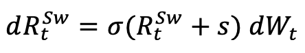
That ensures us that the process remain positive and we can use the Black Formula as in the previous case:
With  and
and  . s is chosen in such a way that
  stays strictly positive.
We can see that the diffusion of is:
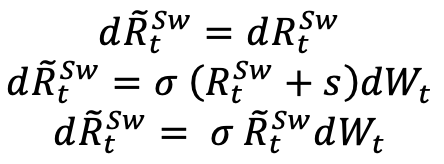
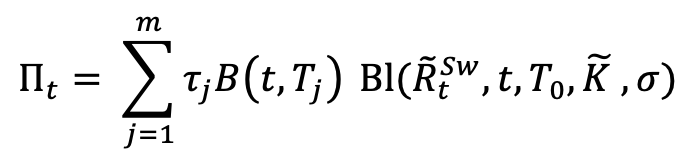
So follows a Black log-normal diffusion and we can price the swaption with the Black formula:
In the case of negative interest rates, the market does not provide the log-normal vol as before but the normal vol. This vol is the implied volatility deduced from the price of swaptions where it is supposed that the forward swap rate follows a normal diffusion:
![]()
Contrary to the Black model, the normal model allows the swap rate to take negative values. To find the volatility, the process is the same as in the case of non-negative interest rates but with an extra stage.
From the normal volatility, we deduce the price of the swaptions for each duration and each exercise time. We then calculate the log-normal volatility of from these prices. Then, the process is the same as in the case of non-negative swap rates.
We finally have volatility surfaces for each duration for the log-normal process and we use it to price our swaption.
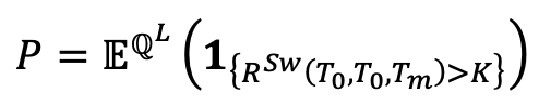
What we call the Exercise Probability is: ![]()
where we suppose: t = 0.
We have:
So:
![]()
With the same notations as previously.