Pricing Constant Maturity Swaps, Swaps and Caps

For pricing constant maturity swaps (CMS), swaps and caps, and especially how convexity adjustment is managed, Finance Active uses the method developed by Patrick Hagan in his article Convexity Conundrums: Pricing CMS Swaps, Caps and Floors.

In our notation, today is always t = 0.

Let's consider:

• A CMS swap leg paying the N year swap rate.
• j = 1, 2, …, m

For each period j, the CMS leg pays:

paid at

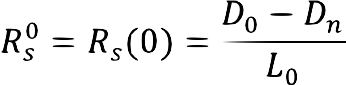
The level of the swap is defined as:

The forward swap rate is:

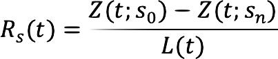
In particular, today’s level is:

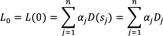
And today’s swap rate is:

We begin with the pricing of a CMS caplet. The payoff of a CMS caplet with a fixing date τ is:

paid at

From the fundamental formula of the pricing, today’s value of the caplet is (under the level numeraire):

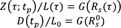
The ratio Z(τ;)/L(τ) is a martingale under the level numeraire, so its average value is today’s value:

By dividing Z(τ; )⁄L(τ) by its mean, we get:

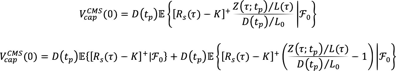
The first term is the price of a European swaption with the notional D()⁄. The last term is the convexity correction.

There are two steps in evaluating the convexity correction. The first step is to model the yield curve movement in a way that allows us to rewrite the level L(τ) and the zero-coupon bond Z(τ;) in terms of the swap rate . Then we can write:

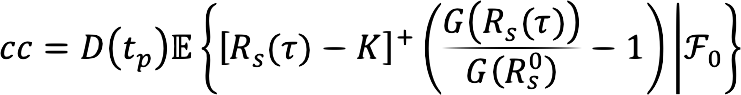
For some G() functions, the convexity correction is just the expected value:

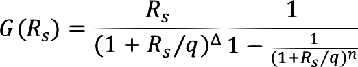
The function we use is called standard model (or street-standard model) in Hagan's article:

The second step is to replicate the payoff in terms of payer swaptions. For any smooth functions f() with f(K)=0, we can write:

Choosing:

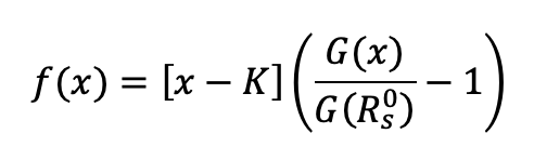
We get:

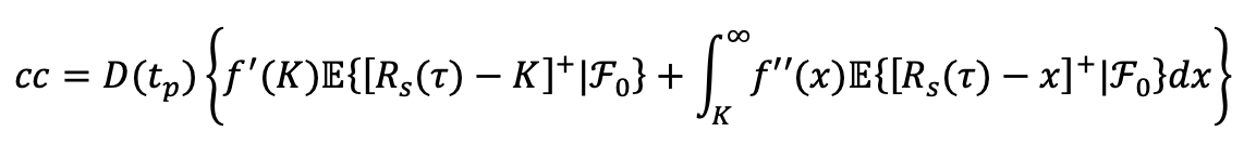
So we get for the value of the CMS caplet:

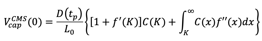
With the value of a payer swaption with strike x:

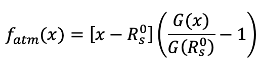
With similar arguments, we get the value of a CMS floorlet:

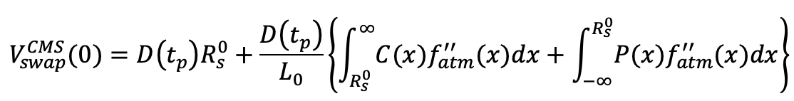
With the same as f(x) with the strike K replaced by the swap rate :

The values C(x) and P(x) are computed with our internal swaption volatility surfaces, built when supposing the forward swap rate is following the SABR model.